Random Walks and Their Convergence

Distances to equilibrium · spectral gap · mixing times · canonical paths

CMSC 35410 · Lecture 3

§0 Where we are

Recap: Lecture 2

\(G = (V,E,w)\) undirected, connected; \(\pi_i = d_i/\mathrm{vol}(V)\); \(P = D^{-1}A\); random-walk Laplacian \(L_{rw} = D^{-1}L = I - P\).

Graphs as differential operators. \(L = \nabla^*\nabla\) and \(L_{rw} = \nabla_\pi^*\nabla\) (up to \(\mathrm{vol}(V)\)): the same \(-\operatorname{div}\nabla\) with different vertex measures. Dirichlet form \[\mathcal E(f,g) = \langle f,L_{rw}g\rangle_\pi = \tfrac{1}{\mathrm{vol}(V)}\textstyle\sum_{\{i,j\}\in E}w_{ij}(f_i-f_j)(g_i-g_j).\]

The walk. Heat kernel \(H_t = e^{-tL_{rw}}\): measures evolve as \(\mu_t^\top = \mu_0^\top H_t\), functions as \(f_t = H_tf\). Detailed balance makes \(H_t\) self-adjoint in \(L^2(\pi)\), so densities \(h_t = \mu_t/\pi\) obey \(h_t = H_th_0\).

The gap. Eigenbasis \(\varphi_1 = \mathbf 1,\dots,\varphi_n\) of \(L_{rw}\) in \(L^2(\pi)\), \(0 = \lambda_1<\lambda_2\le\dots\le\lambda_n\le2\). Spectral gap \(\lambda := \lambda_2\) = best constant in Poincaré: \(\lambda\operatorname{Var}_\pi(f)\le\mathcal E(f,f)\). Relaxation time \(t_{\rm rel} = 1/\lambda\).

~5 min. Everything today happens in L²(π): we track the density h_t = μ_t/π, which evolves by the same heat kernel as functions. That is what lets us measure convergence with Var_π, Ent_π, and the Dirichlet form. Recall the split-and-aggregate demo: μ_t → π (uneven, ∝ degree) while h_t → 1 (flat).

Today

How fast does the walk forget where it started?

1. How to measure convergence: \(\ell_1\), \(\chi^2\), entropy. Mixing time.
2. Spectral gap \(\Rightarrow\) exponential decay of \(\chi^2\); the heat flow as a gradient flow.
3. Consequences for \(\ell_1\) and entropy (→ log-Sobolev, later).
4. Cycle, grid, binary tree: upper and lower bounds on the gap; how tight is all this?

§1 · Measuring convergence

Three distances to \(\pi\)

For \(\mu\) with density \(h = \mu/\pi\):

	measure form	density form
TV	\(\|\mu-\pi\|_{TV} = \tfrac12\|\mu-\pi\|_1 = \max_S|\mu(S)-\pi(S)|\)	\(\tfrac12\,\mathbb E_\pi|h-1|\)
\(\boldsymbol{\chi^2}\)	\(\chi^2(\mu\Vert\pi) = \sum_i\frac{(\mu_i-\pi_i)^2}{\pi_i} = \|\mu-\pi\|^2_{1/\pi}\)	\(\operatorname{Var}_\pi(h)\)
KL	\(D(\mu\Vert\pi) = \sum_i\mu_i\log\frac{\mu_i}{\pi_i}\)	\(\operatorname{Ent}_\pi(h)\)

All of the form \(\mathbb E_\pi\Phi(h)\), \(\Phi\) convex, \(\Phi(1) = 0\): \(\;\tfrac12|x-1|,\ (x-1)^2,\ x\log x\).

From a point mass \(\delta_x\), on a bounded-degree graph (\(\pi_x\approx1/n\)):

\[ \|\delta_x-\pi\|_{TV} = 1-\pi_x\le1,\qquad D(\delta_x\Vert\pi) = \log\tfrac1{\pi_x}\approx\log n,\qquad\chi^2(\delta_x\Vert\pi) = \tfrac1{\pi_x}-1\approx n . \]

Remember \(1\) vs. \(\log n\) vs. \(n\). It is the whole story of §3.

How they compare

We will directly bound the total variation distance in terms of \(\chi^2\) and KL divergences using the lemmata 1 and 2 below. We will use lemma 3 to bound the KL divergence in terms of \(\chi^2\).

Lemma. For every \(\mu\):

1. \(\|\mu-\pi\|_{TV}\le \frac{1}{2} \sqrt{\chi^2(\mu\Vert\pi)}\)
2. (Pinsker) \(\|\mu-\pi\|_{TV}\le\sqrt{\tfrac12D(\mu\Vert\pi)}\)
3. \(D(\mu\Vert\pi)\le\log\big(1+\chi^2(\mu\Vert\pi)\big)\le\chi^2(\mu\Vert\pi)\)

Proofs.

1. Cauchy–Schwarz in \(L^2(\pi)\): \[\begin{align*} \|\mu-\pi\|_{TV} &= \frac{1}{2} \mathbb{E}_\pi\big[|h-1|\big] \le \frac{1}{2} \sqrt{\mathbb{E}_\pi\big[(h-1)^2\big] \cdot \mathbb{E}_\pi[1]} \\ &= \frac{1}{2} \sqrt{\chi^2(\mu\Vert\pi)}. \end{align*}\] Because \(\mathbb{E}_\pi[1] = 1\) and \(\mathbb{E}_\pi[h] =1\), so that \(\mathbb{E}_\pi\big[(h-1)^2\big] = \operatorname{Var}_\pi [h] = \chi^2(\mu\Vert\pi)\), the inequality follows.

2. I prefer to think of this as a consequence of the strong convexity wrt the \(\ell_1\) norm of the entropy function over probability densities. By Taylor’s theorem, we have the expansion:

\[\begin{align*} D(\mu\Vert\pi) &= \operatorname{Ent}_\pi(h) = \operatorname{Ent}_\pi(1) + \langle \nabla \operatorname{Ent}_\pi(1), h-1\rangle_\pi \\&+ \frac{1}{2} \langle h-1, \nabla^2 \operatorname{Ent}_\pi(\xi)(h-1)\rangle_\pi \end{align*}\]

But \(\operatorname{Ent}_\pi(1) = 0\) and \(\nabla \operatorname{Ent}_\pi(1) = 0\), so that the first two terms vanish. Furthermore: \[ \nabla^2 \operatorname{Ent}_\pi(\xi) = \mathrm{diag}\Big(\frac{1}{\xi}\Big). \] By Cauchy–Schwarz, we get: \[\begin{align*} D(\mu\Vert\pi) &= \frac{1}{2} \langle h-1, \nabla^2 \operatorname{Ent}_\pi(\xi)(h-1)\rangle_\pi \geq \frac{\Big(\mathbb{E}_\pi \|h-1\|_{1}\Big)^2}{2 \mathbb{E}_\pi[\xi]} \\ &= 2\|\mu-\pi\|_{TV}^2. \end{align*}\]

3. Jensen for concave \(\log\) under \(\mu\): \(\|\mu - \pi\|_{TV} = \frac{1}{2} \sqrt{\chi^2(\mu\Vert\pi)}\). \[ D = \mathbb E_\mu\log h\le\log\mathbb E_\mu h = \log\mathbb E_\pi h^2 = \log(1+\operatorname{Var}_\pi h). \]

explain gradient, nablaEnt is wrong and check 2.

Monotone — but at what rate?

Lemma. For convex \(\Phi:\mathbb R\to\mathbb R\) (applied pointwise, as on the previous slide), \(t\mapsto\mathbb E_\pi\Phi(H_th)\) is non-increasing.

Proof. Jensen pointwise, \(\Phi(H_th)\le H_t\Phi(h)\); stationarity, \(\mathbb E_\pi H_tg = \mathbb E_\pi g\). \(\square\) (For TV: the \(\ell_1\) contraction exercise.)

TV is the distance we want. \(\boldsymbol{\chi^2}\) and entropy are the ones we can differentiate along the flow and close with a functional inequality.

Mixing time: worst case over starting vertices; by convexity of the distance, this is also the worst case over all starting distributions.

\[ d(t) := \max_x\|\delta_xH_t - \pi\|_{TV},\qquad t_{\rm mix}(\varepsilon) := \min\{t: d(t)\le\varepsilon\}, \]

\[ t_{\rm mix} := t_{\rm mix}(\tfrac14). \]

Same with \(\sqrt{\chi^2}\) (\(\ell^2\)-mixing) or \(D\) (entropy mixing). Discrete/lazy: replace \(H_t\) by \(P_{\rm lazy}^t\).

Convexity: μ = Σ_x μ_x δ_x and H_t is linear, so ‖μH_t − π‖ = ‖Σ_x μ_x(δ_x H_t − π)‖ ≤ Σ_x μ_x ‖δ_x H_t − π‖ ≤ max_x ‖δ_x H_t − π‖ (TV is a norm; χ² and KL are convex f-divergences). A convex function on the simplex is maximized at a vertex = a point mass.

d(t) is essentially submultiplicative, so t_mix(ε) ≤ ⌈log2(1/ε)⌉ t_mix (LPW Ch. 4): 1/4 is just a convention.

Monotone, again: by differentiating

\(h_t = H_th\) satisfies \(\partial_th_t = -L_{rw}h_t\). Differentiate \(\mathbb E_\pi\Phi(h_t)\) directly:

\[ \frac{d}{dt}\mathbb E_\pi\Phi(h_t) = \mathbb E_\pi\big[\Phi'(h_t)\,\partial_th_t\big] = -\langle\Phi'(h_t),L_{rw}h_t\rangle_\pi = -\mathcal E\big(\Phi'(h_t),h_t\big). \]

\[ \mathcal E(\Phi'(h_t),h_t) = \frac1{\mathrm{vol}(V)}\sum_{\{i,j\}\in E}w_{ij}\big(\Phi'(h_i)-\Phi'(h_j)\big)(h_i-h_j). \]

Convex \(\Phi\) \(\Rightarrow\) \(\Phi'\) non-decreasing \(\Rightarrow\) every term \(\ge0\) (same-signed factors). Hence

\[ \frac{d}{dt}\mathbb E_\pi\Phi(h_t) = -\mathcal E(\Phi'(h_t),h_t)\ \le\ 0. \qquad\square \]

Same template, two more times:

• \(\Phi(x)=(x-1)^2\): \(\Phi'(x)=2(x-1)\), recovering Proof 2 below, exactly.
• \(\Phi(x)=x\log x\): \(\Phi'(x)=\log x+1\), recovering the entropy-production formula of §3.

Needs Φ differentiable — doesn’t cover TV (Φ(x) = |x-1|/2 is not differentiable at x=1), which is why the Monotone slide still cites the ℓ1-contraction exercise for that case. Key fact used for the sign: convex ⟺ Φ’ non-decreasing ⟺ (Φ’(a)-Φ’(b))(a-b) ≥ 0 for all a,b. This is the one-line generalization of “Proof 2: the template for the rest of the course” coming up: same differentiate-and-use-the-Dirichlet-form move, here for the qualitative statement (monotone decrease), there (Φ = (x-1)²) for the quantitative rate via Poincaré.

§2 · Spectral gap ⇒ χ² decay

The theorem

Theorem. For all \(h\) and \(t\ge0\): \[\operatorname{Var}_\pi(H_th)\le e^{-2\lambda t}\operatorname{Var}_\pi(h),\qquad\text{i.e.}\qquad\chi^2(\mu_t\Vert\pi)\le e^{-2\lambda t}\chi^2(\mu_0\Vert\pi).\] Sharp: equality for \(h = 1+\epsilon\varphi_2\).

Proof 1 (spectral). \[ \operatorname{Var}_\pi(H_th) = \sum_{k\ge2}e^{-2\lambda_kt}\langle h,\varphi_k\rangle_\pi^2\le e^{-2\lambda t}\sum_{k\ge2}\langle h,\varphi_k\rangle_\pi^2 . \qquad\square \]

Proof 2: the template for the rest of the course

\(h_t = H_th\); \(\;\mathbb E_\pi h_t\equiv c\) is conserved. Then

\[ \frac{d}{dt}\operatorname{Var}_\pi(h_t) = 2\langle h_t - c,\ \partial_th_t\rangle_\pi = -2\langle h_t - c, L_{rw}h_t\rangle_\pi = -2\,\mathcal E(h_t,h_t). \]

Variance dissipates at rate \(2\mathcal E\). Poincaré: \(\mathcal E\ge\lambda\operatorname{Var}\), so \(\frac d{dt}\operatorname{Var}\le-2\lambda\operatorname{Var}\); Grönwall. \(\square\)

No diagonalization. Only: (dissipation identity) + (functional inequality).

• (Var, Poincaré) \(\to\) \(\chi^2\) decay at rate \(2\lambda\). (Today.)
• (Ent, log-Sobolev) \(\to\) entropy decay. (§3, then later.)
• Graph \(\to\) manifold: Bakry–Émery. (Later.)

Conversely, decay at rate \(2c\) for all \(h\) \(\Rightarrow\) differentiate at \(t=0\) \(\Rightarrow\) \(c\le\lambda\). Gap = optimal \(\chi^2\) rate.

The heat flow is a gradient flow

Geometry: densities in \(L^2(\pi)\), where the distance to equilibrium is \(\|h-1\|_\pi^2 = \chi^2(\mu\Vert\pi)\). Energy: \(F(h) := \tfrac12\mathcal E(h,h) = \tfrac12\,\|\nabla h\|_w^2/\mathrm{vol}(V)\).

Gradient. \(F(h+\epsilon v) = F(h) + \epsilon\,\mathcal E(h,v) + O(\epsilon^2) = F(h) + \epsilon\,\langle L_{rw}h, v\rangle_\pi + O(\epsilon^2)\), so

\[ \nabla_\pi F(h) = L_{rw}h \qquad\Longrightarrow\qquad \partial_th_t = -\nabla_\pi F(h_t) = -L_{rw}h_t , \]

which is the heat equation for densities from Lecture 2. Heat flow = steepest descent of the energy in the \(\chi^2\) geometry.

Poincaré = strong convexity. \(F(h)\ge\frac\lambda2\|h-\mathbb E_\pi h\|_\pi^2\): the energy is \(\lambda\)-strongly convex transverse to its minimizers (the constants). The gradient flow of a \(\lambda\)-strongly convex function contracts the squared distance to its minimizer at rate \(2\lambda\): this is the \(\chi^2\) theorem. Proof 2 was exactly this computation, \(\frac{d}{dt}\tfrac12\|h_t-1\|_\pi^2 = -\langle h_t-1,\nabla_\pi F(h_t)\rangle_\pi = -2F(h_t)\).

Aside: \(\mathcal E\) is a dissipative bracket. In the language of GENERIC/metriplectic dynamics (Grmela–Öttinger; Morrison), \(\mathcal E\) is symmetric, PSD, and degenerate on the conserved quantity — \(\mathcal E(f,\mathbf 1)=0\) since \(L_{rw}\mathbf1=0\) — exactly the axioms of a dissipative bracket. No Jacobi identity: that’s the axiom of the other, antisymmetric Poisson-bracket half of such systems, which is simply absent here — the heat flow is pure dissipation, no reversible/Hamiltonian part.

Discretizing time: \(h_{k+1} = \arg\min_h\Big\{F(h) + \frac{1}{2\tau}\|h-h_k\|_\pi^2\Big\} = (I+\tau L_{rw})^{-1}h_k\ \to\ H_th_0\) as \(\tau\to0\).

Question: is there a geometry in which the heat flow is the gradient flow of the entropy, and does convexity of the entropy give entropy decay?

χ² is the natural convergence measure for the heat flow because it is the squared norm of the Hilbert space in which the heat flow is a gradient flow; the gap is the strong-convexity modulus of the energy in that space. Minimizing movement: first-order condition L_rw h + (h − h_k)/τ = 0, i.e. implicit Euler. Answer to the question (for later): yes. On R^n, Jordan–Kinderlehrer–Otto (SIAM J. Math. Anal. 1998): the Fokker–Planck/heat flow is the gradient flow of relative entropy w.r.t. the Wasserstein-2 metric; λ-geodesic convexity of entropy (Bakry–Émery / Ricci ≥ λ) ⇒ LSI ⇒ entropy decay. On finite Markov chains, W2 fails (no geodesics through discrete measures); Maas (J. Funct. Anal. 2011) and Mielke (Nonlinearity 2011) built a discrete transport metric in which the continuous-time chain is the gradient flow of entropy; Erbar–Maas (2012): entropic Ricci curvature ≥ κ ⇒ MLSI with ρ₀ ≥ 2κ. (Citation details from memory: check.)

On the dissipative-bracket aside: GENERIC splits dynamics as dx/dt = {x,E} + (x,S), Poisson bracket {.,.} antisymmetric and satisfying Jacobi (reversible, energy-conserving part), dissipative bracket (.,.) symmetric and semi-definite with (E,.)=0 (irreversible, entropy-producing part). Here there is no Poisson half at all — partial_t h_t = -L_rw h_t is pure gradient descent, no Hamiltonian term — so this is a maximally degenerate GENERIC system: all dissipation, no symplectic structure. The entropy-production identity d/dt E_pi Phi(h_t) = -E(Phi’(h_t), h_t), shown on “Monotone, again: by differentiating”, is exactly the GENERIC formula dS/dt = (dS,dS) for this bracket. References: Grmela & Öttinger, “Dynamics and thermodynamics of complex fluids I” (Phys. Rev. E, 1997); P. Morrison, “Some observations regarding brackets and dissipation” (1984), who coined “metriplectic.” (Citation details from memory: check.)

Discrete time

• Lazy chain: \(\operatorname{Var}_\pi(P_{\rm lazy}^th)\le(1-\tfrac\lambda2)^{2t}\operatorname{Var}_\pi(h)\).
• Non-lazy: factor \(\lambda_\star^{2t}\), \(\;\lambda_\star = \max_{k\ge2}|1-\lambda_k|\) — equal to \(1\) on bipartite graphs.

§3 · Consequences for ℓ₁ and entropy

The gap pins down the mixing time

Theorem. For the continuous-time walk, \(\pi_{\min} = \min_x\pi_x\): \[ \frac1\lambda\log\frac1{2\varepsilon}\ \le\ t_{\rm mix}(\varepsilon)\ \le\ \frac1\lambda\Big(\tfrac12\log\frac1{\pi_{\min}} + \log\frac1{2\varepsilon}\Big). \]

Upper. Lemma (1) + §2: \(\;\|\delta_xH_t-\pi\|_{TV}\le\tfrac12\sqrt{\chi^2(\delta_xH_t\Vert\pi)}\le\tfrac12e^{-\lambda t}\pi_x^{-1/2}\).

Lower. Scale \(f = \varphi_2\) so \(\|f\|_\infty = 1 = |f(x)|\). Then \(\mathbb E_\pi f = 0\), \((H_tf)(x) = e^{-\lambda t}f(x)\), and \[ e^{-\lambda t} = |\mathbb E_{\delta_xH_t}f - \mathbb E_\pi f|\le\|\delta_xH_t-\pi\|_1\|f\|_\infty = 2\|\delta_xH_t-\pi\|_{TV}. \qquad\square \]

Lazy discrete version: (2/λ − 1) log(1/2ε) ≤ t_mix(ε) ≤ (2/λ)(½ log(1/π_min) + log(1/2ε)); lower bound uses log(1/(1−x)) ≤ x/(1−x). Cf. LPW Thms 12.4–12.5 (check numbering).

Where the \(\log(1/\pi_{\min})\) comes from

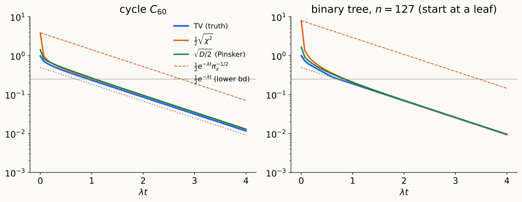
\(\chi^2\) starts at \(\approx n\) and must spend time \(\approx\frac{\log n}{2\lambda}\) just getting below \(1\). TV starts at \(\le1\).

x-axis in units of t_rel. TV (blue) stays sandwiched between the lower bound (grey dotted) and the χ²-bound (orange dashed). The orange solid χ² curve only drops below 1/4 well after TV. Entropy (green) starts at log n, much lower than n.

Entropy along the flow

Same computation as Proof 2, with \(\operatorname{Ent}_\pi\) in place of \(\operatorname{Var}_\pi\):

\[ \frac d{dt}\operatorname{Ent}_\pi(h_t) = \mathbb E_\pi\big[(1+\log h_t)\,\partial_th_t\big] = -\langle\log h_t, L_{rw}h_t\rangle_\pi \]

\[ = -\mathcal E(h_t,\log h_t)\ \le\ 0 . \]

\(\mathcal E(h,\log h)\): entropy production (discrete Fisher information).

From the gap alone (Lemma 3): \(\;D(\mu_t\Vert\pi)\le\log\big(1 + e^{-2\lambda t}\chi^2(\mu_0\Vert\pi)\big)\) — rate \(2\lambda\) eventually, but the same \(\log n\) burn-in.

To close the loop we need a new functional inequality, the modified log-Sobolev inequality:

\[ \rho_0\operatorname{Ent}_\pi(h)\le\mathcal E(h,\log h)\quad\Longrightarrow\quad D(\mu_t\Vert\pi)\le e^{-\rho_0t}D(\mu_0\Vert\pi). \]

Preview: log-Sobolev trades \(\log n\) for \(\log\log n\)

With Pinsker:

\[ t_{\rm mix}(\varepsilon)\le\frac1{\rho_0}\Big(\log\log\frac1{\pi_{\min}} + \log\frac1{2\varepsilon^2}\Big) \qquad\text{vs.}\qquad \frac1\lambda\Big(\tfrac12\log\frac1{\pi_{\min}} + \log\frac1{2\varepsilon}\Big). \]

The price is the constant: entropy can’t decay faster than twice the gap,

\[ \rho_0\ \le\ 2\lambda . \]

Proof. Linearize at equilibrium, \(h = 1+\epsilon g\), \(\mathbb E_\pi g = 0\): \[ \operatorname{Ent}_\pi(h) = \tfrac{\epsilon^2}2\operatorname{Var}_\pi g + O(\epsilon^3),\qquad \mathcal E(h,\log h) = \epsilon^2\mathcal E(g,g) + O(\epsilon^3). \] MLSI forces \(\rho_0\le 2\,\mathcal E(g,g)/\operatorname{Var}_\pi g\) for every \(g\); take \(g = \varphi_2\). \(\square\)

Entropy wins when \(\rho_0\) is comparable to the gap. When is it? How do we bound it? → later lecture.

Say aloud: next time we meet the classical log-Sobolev inequality α Ent(f²) ≤ E(f,f) (Gross), which is how ρ₀ is bounded in practice (it tensorizes; ρ₀ ≥ 4α via (a−b)(log a − log b) ≥ 4(√a−√b)²), and which coincides with this one for diffusions (chain rule: E(h, log h) = 4E(√h,√h) exactly). If asked for a lower bound in terms of λ: Diaconis–Saloff-Coste give α ≥ (1−2π_)λ / log(1/π_ − 1), so ρ₀ ≳ 4λ/log(1/π_min) — plugging it in is worse than the gap bound by log log, so the gap alone never certifies that entropy helps. K_n: λ ≍ 1, α ≍ 1/log n, ρ₀ ≍ 1 (Bobkov–Tetali). (Constants from memory — check.)

§4 · Examples: the gap from both sides

Toolkit

Upper bounds: test functions. Any non-constant \(f\): \(\;\lambda\le\mathcal E(f,f)/\operatorname{Var}_\pi(f)\). Make \(f\) change slowly across a bottleneck.

Degree comparison. If \(d_{\min}\le d_i\le d_{\max}\):

\[ \frac{\lambda_2(L)}{d_{\max}}\le\lambda = \lambda_2(L_{rw})\le\frac{\lambda_2(L)}{d_{\min}}. \]

(Both are \(\min_f f^\top Lf\,/\min_c\|f-c\|_m^2\), with \(m = d\) vs. \(m = \mathbf 1\).) Our examples have \(1\le d\le4\): work with \(L\).

Lower bounds: canonical paths — the discrete version of the 1-D Poincaré proof:

\[ f(b)-f(a) = \int_a^bf'\quad+\quad\text{Cauchy–Schwarz}. \]

Canonical paths

For each ordered pair \((a,b)\) choose a path \(\gamma_{ab}\); choose edge lengths \(\ell_e>0\) (default \(\ell\equiv1\)). Congestion:

\[ \kappa := \max_{e\in E}\ \frac1{w_e\ell_e}\sum_{(a,b):\,e\in\gamma_{ab}}\ell(\gamma_{ab}),\qquad\ell(\gamma) = \sum_{e\in\gamma}\ell_e . \]

Theorem (Jerrum–Sinclair; Diaconis–Stroock). \(\;\sum_{a,b}(f_a-f_b)^2\le\kappa\,f^\top Lf\), hence \(\;\lambda_2(L)\ge\dfrac{2n}\kappa\).

Proof. \((f_b - f_a)^2 = \big(\sum_{e\in\gamma_{ab}}\nabla_ef\big)^2\le\ell(\gamma_{ab})\sum_{e\in\gamma_{ab}}\frac{(\nabla_ef)^2}{\ell_e}\). Sum over pairs, swap sums:

\[ \sum_{a,b}(f_a-f_b)^2\le\sum_ew_e(\nabla_ef)^2\cdot\underbrace{\frac{1}{w_e\ell_e}\sum_{\gamma_{ab}\ni e}\ell(\gamma_{ab})}_{\le\kappa},\qquad\sum_{a,b}(f_a-f_b)^2 = 2n\|f-\bar f\|^2 . \ \square \]

π-weighted version, directly for λ: Var_π f = ½ Σ π_a π_b (f_a − f_b)², E(f,f) = Σ_e Q(e)(∇e f)², Q(e) = w_e/vol. Same proof: λ ≥ 1/κ_π, κ_π = max_e (1/(Q(e) ℓ_e)) · ½ Σ{γ_ab ∋ e} π_a π_b ℓ(γ_ab). Interpretation: κ is the congestion of an (unsplittable) multicommodity flow routing one unit between every pair. A bottleneck forces congestion — paths certify the absence of bottlenecks, dual to the test-function certificate. Flow/cut duality → Cheeger next week, Leighton–Rao later.

Cycle \(C_n\)

Exact (Fourier): \(L\) has eigenvalues \(2-2\cos(2\pi j/n)\); since \(D = 2I\), \(\;L_{rw} = L/2\) and \[\lambda = 1-\cos\tfrac{2\pi}n = 2\sin^2\tfrac\pi n\approx\frac{2\pi^2}{n^2}\approx\frac{19.7}{n^2}.\]

Canonical paths (\(n = 2m+1\), shortest paths, \(\ell\equiv1\)): each vertex has 2 vertices at each distance \(s = 1,\dots,m\). By rotation symmetry all edges carry equal load:

\[ \kappa = \frac1n\sum_{(a,b)}|\gamma_{ab}|^2 = 2\sum_{s=1}^ms^2 = \frac{n(n^2-1)}{12} \qquad\Longrightarrow\qquad \lambda_2(L)\ge\frac{2n}{\kappa} = \frac{24}{n^2-1}. \]

Divide by \(d = 2\) to compare with the exact \(\lambda\): \[ \frac{12}{n^2-1}\ \le\ \lambda\ \approx\ \frac{19.7}{n^2}. \] Right order; constant \(12\) vs. \(2\pi^2\approx19.7\).

Σ_e load(e) = Σ_{(a,b)} |γ_ab|² because each pair contributes |γ| to each of its |γ| edges. Careful with normalizations: λ₂(L) = 2λ ≈ 4π²/n² ≈ 39.5/n² ≥ 24/(n²−1); for λ = λ₂(L_rw): 12/(n²−1) ≤ 2π²/n².

The \(k\times k\) grid, \(n = k^2\)

Test function \(f(x,y) = x - \frac{k+1}2\): only horizontal edges see a difference (each 1),

\[ \lambda_2(L)\le\frac{k(k-1)}{k\cdot k(k^2-1)/12} = \frac{12}{k(k+1)},\qquad\lambda\le\frac{6}{k(k+1)}\ \ (d_{\min} = 2). \]

Canonical paths, “L-shaped”: horizontal along \(a\)’s row to \(b\)’s column, then vertical. Length \(\le2(k-1)\).

• horizontal edge, row \(r\), between columns \(c|c+1\): needs \(a\) in row \(r\), \(a_x\) and \(b_x\) on opposite sides: \(\;2\,c(k-c)\,k\le k^3/2\) pairs;
• vertical edge, column \(c\), between rows \(r|r+1\): needs \(b\) in column \(c\), \(a_y,b_y\) on opposite sides: \(\;2\,r(k-r)\,k\le k^3/2\) pairs.

\[ \kappa\le\frac{k^3}2\cdot2(k-1)\quad\Longrightarrow\quad\lambda_2(L)\ge\frac{2}{k(k-1)},\qquad\lambda\ge\frac1{2k(k-1)}\ \ (d_{\max} = 4). \]

So \(\lambda = \Theta(1/k^2) = \Theta(1/n)\). (Exact: \(\lambda_2(L) = 2-2\cos\frac\pi k\approx\frac{\pi^2}{k^2}\), via \(L(G\,\square\,H) = L_G\otimes I + I\otimes L_H\) and the Neumann cosines of the path.)

Binary tree, depth \(h\), \(n = 2^{h+1}-1\): upper bound

Test function: \(+1\) on the left subtree, \(-1\) on the right, \(0\) at the root.

• \(\mathbb E_\pi f = 0\) by symmetry;
• only the two root edges see a difference: \(\sum w(\nabla f)^2 = 2\);
• \(\sum_id_if_i^2 = \mathrm{vol}(V) - d_{\rm root} = 2(n-1)-2\).

\[ \lambda\le\frac{2}{2n-4} = \frac1{n-2}. \]

The root is a bottleneck: two edges separate two halves of size \(\approx n/2\). (Cheeger next week: conductance \(\approx 2/n\).)

Binary tree: lower bound, and choosing lengths

Paths are forced. An edge at depth \(j\) cuts off \(s_j = 2^{h-j+1}-1\) vertices: used by \(2s_j(n-s_j)\le n^2/2\) ordered pairs.

Unit lengths: \(|\gamma|\le2h\), so \(\kappa\le n^2h\) and \(\;\lambda_2(L)\ge\dfrac{2}{nh}\) — off by \(\log_2n\). Cauchy–Schwarz charges every edge of a long path equally, but only the top edges are congested.

Weighted lengths \(\ell_e = 2^{-j/2}\) at depth \(j\) (cheap where congested): \(\ell(\gamma)\le2\sum_{j\ge1}2^{-j/2} = 2(\sqrt2+1)\), and with \(s_j<(n+1)2^{-j}\),

\[ \frac1{\ell_e}\sum_{\gamma\ni e}\ell(\gamma)\le2^{j/2}\cdot2s_jn\cdot2(\sqrt2+1) < 2(2+\sqrt2)\,n(n+1) \quad\Longrightarrow\quad \lambda_2(L) > \frac{1}{(2+\sqrt2)(n+1)}. \]

With \(d\le3\): \(\;\dfrac{1}{3(2+\sqrt2)(n+1)}<\lambda\le\dfrac1{n-2}\), so \(\lambda = \Theta(1/n)\).

The choice of ℓ is the discrete analog of the weight in a weighted Poincaré / Hardy inequality. Numerically n·λ → ≈ 0.5 for the binary tree.

Bounds vs. truth

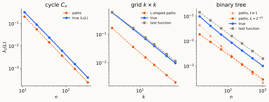
Parallel lines = right order. Unit-length paths on the tree drift away by \(\log n\).

How tight are the convergence bounds?

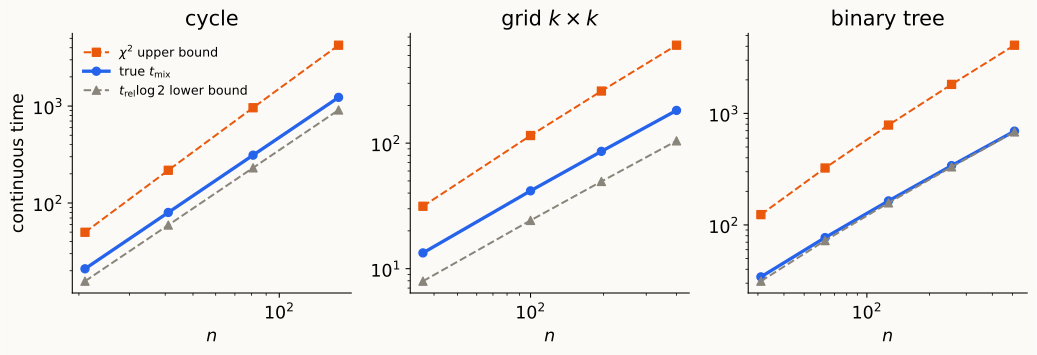
	\(t_{\rm rel}\)	\(\chi^2\) upper bound	true \(t_{\rm mix}\)
cycle	\(\Theta(n^2)\)	\(\Theta(n^2\log n)\)	\(\Theta(n^2)\)
grid	\(\Theta(n)\)	\(\Theta(n\log n)\)	\(\Theta(n)\)
binary tree	\(\Theta(n)\)	\(\Theta(n\log n)\)	\(\Theta(n)\)

Lower bound tight on all three; the generic χ² upper bound loses exactly log n. Numbers: C_161: t_mix ≈ 1230, lower 910, upper 4247. Tree n=1023: 1402 vs lower 1388 (!) vs upper 9022.

The loss is not in \(\chi^2\) — it is in using only \(\lambda_2\)

Exactly, from the spectral expansion of \(h_0 = \mathbf 1_x/\pi_x\):

\[ \chi^2(\delta_xH_t\Vert\pi) = \sum_{k\ge2}e^{-2\lambda_kt}\varphi_k(x)^2,\qquad\sum_k\varphi_k(x)^2 = \frac1{\pi_x}. \]

The generic bound pretends all \(n-1\) modes decay as slowly as \(\varphi_2\).

Vertex-transitive graphs: \(\chi^2(\delta_xH_t\Vert\pi) = \sum_{k\ge2}e^{-2\lambda_kt}\). Cycle: \(1-\cos\theta\ge\frac{2\theta^2}{\pi^2}\) gives

\[ \chi^2(\delta_xH_t\Vert\pi)\le2\sum_{j\ge1}e^{-16tj^2/n^2} = O(1)\quad\text{at } t = \Theta(n^2). \]

So even \(\ell^2\)-mixing on the cycle is \(\Theta(n^2)\), not \(n^2\log n\).

Preview: when even \(t_{\rm rel}\) is not the answer

Hypercube \(\{0,1\}^d\), \(n = 2^d\) (flip a uniform coordinate at rate 1): eigenvalues \(\frac{2|S|}d\), \(S\subseteq[d]\), so \(t_{\rm rel} = d/2\), and exactly

\[ \chi^2(\delta_xH_t\Vert\pi) = \big(1+e^{-4t/d}\big)^d - 1 \]

which is \(O(1)\) iff \(t\ge\frac d4\log d - O(d)\). TV has a cutoff at the same time (Diaconis; LPW).

	lower: \(t_{\rm rel}\)	upper: \(\chi^2\) + gap	upper: entropy + LSI	truth
hypercube	\(\Theta(d)\)	\(\Theta(d^2)\)	\(\Theta(d\log d)\)	\(\sim\frac d4\log d\)

LSI constant \(\Theta(1/d)\) (tensorization), and \(\log\log(1/\pi_{\min}) = \log(d\log2)\): tight. The motivating example for log-Sobolev inequalities.

Takeaways

• Want TV; differentiate \(\chi^2\) and entropy: dissipation identity + functional inequality.
• Gap = optimal \(\chi^2\) rate; \(\;t_{\rm rel}\log\frac1{2\varepsilon}\le t_{\rm mix}(\varepsilon)\le t_{\rm rel}\big(\frac12\log\frac1{\pi_{\min}}+\log\frac1{2\varepsilon}\big)\).
• Bound the gap with test functions (above) and canonical paths (below).
• Next: Cheeger — when do test functions and paths meet?

Appendix: definitions for the board

Operators and the walk

Graph. \(G = (V,E,w)\) undirected, connected; \(d_i = \sum_jw_{ij}\); \(\mathrm{vol}(S) = \sum_{i\in S}d_i\); \(\pi_i = d_i/\mathrm{vol}(V)\), \(\Pi = \operatorname{diag}(\pi)\).

Gradient / divergence. \((\nabla f)(i\to j) = f_j - f_i\); \(\operatorname{div}_m = -\nabla_m^*\) w.r.t. \(\langle\cdot,\cdot\rangle_w\) on edges and \(\langle\cdot,\cdot\rangle_m\) on vertices. \(\nabla^*\nabla = L = D-A\); \(\nabla_d^*\nabla = L_{rw} = D^{-1}L = I-P\); \(\mathcal L = D^{-1/2}LD^{-1/2}\).

Dirichlet form. \(\mathcal E(f,g) = \langle f,L_{rw}g\rangle_\pi = \frac1{\mathrm{vol}(V)}\sum_{\{i,j\}\in E}w_{ij}(f_i-f_j)(g_i-g_j)\).

Walk. \(P = D^{-1}A\); measures \(\mu^\top P\), functions \(Pf\). Random-walk Laplacian \(L_{rw} = I - P\). Continuous time \(H_t = e^{-tL_{rw}}\), generator \(\mathcal A = P - I = -L_{rw}\). Lazy: \(P_{\rm lazy} = \frac12(I+P)\).

Reversibility. \(\Pi P = P^\top\Pi\); densities \(h = \mu/\pi\) evolve as \(h_t = H_th_0\).

Gap / Poincaré. \(\lambda = \lambda_2(L_{rw}) = \min_f\mathcal E(f,f)/\operatorname{Var}_\pi(f)\); \(t_{\rm rel} = 1/\lambda\).

Convergence

Distances. \(\|\mu-\pi\|_{TV} = \frac12\mathbb E_\pi|h-1|\); \(\chi^2(\mu\Vert\pi) = \operatorname{Var}_\pi(h)\); \(D(\mu\Vert\pi) = \operatorname{Ent}_\pi(h)\). \(\;2\,\mathrm{TV}\le\sqrt{\chi^2}\); \(\mathrm{TV}\le\sqrt{D/2}\); \(D\le\log(1+\chi^2)\).

Mixing time. \(d(t) = \max_x\|\delta_xH_t-\pi\|_{TV}\); \(t_{\rm mix}(\varepsilon) = \min\{t: d(t)\le\varepsilon\}\).

χ² decay. \(\operatorname{Var}_\pi(H_th)\le e^{-2\lambda t}\operatorname{Var}_\pi(h)\); \(\frac d{dt}\operatorname{Var}_\pi(h_t) = -2\mathcal E(h_t,h_t)\).

Mixing from the gap. \(\frac1\lambda\log\frac1{2\varepsilon}\le t_{\rm mix}(\varepsilon)\le\frac1\lambda\big(\frac12\log\frac1{\pi_{\min}}+\log\frac1{2\varepsilon}\big)\).

Entropy. \(\frac d{dt}\operatorname{Ent}_\pi(h_t) = -\mathcal E(h_t,\log h_t)\). MLSI \(\rho_0\operatorname{Ent}_\pi(h)\le\mathcal E(h,\log h)\) \(\Rightarrow\) \(D(\mu_t\Vert\pi)\le e^{-\rho_0t}D(\mu_0\Vert\pi)\); \(\;\rho_0\le2\lambda\).

Canonical paths. \(\kappa = \max_e\frac1{w_e\ell_e}\sum_{\gamma_{ab}\ni e}\ell(\gamma_{ab})\) \(\Rightarrow\) \(\lambda_2(L)\ge2n/\kappa\). Degree comparison: \(\lambda_2(L)/d_{\max}\le\lambda\le\lambda_2(L)/d_{\min}\).