Laplacians and Random Walks

Graphs as differential operators · the random walk · measures vs. densities

CMSC 35410 · Lecture 2

§0 Where we are

Last time → today

Lecture 1, §5: heat on a graph, \(\dot u = -Lu\), and on a manifold, \(\partial_t u = -\Delta u\), with \(\Delta = -\operatorname{div}\nabla\). “The Fiedler vector is the last non-uniform heat left.”

Today we make that picture precise:

1. Graph matrices are \(-\operatorname{div}\nabla\) (for the right measures).
2. The random walk and the heat kernel; measures vs. functions; the spectral gap.

Next lecture: how fast the walk converges — distances to \(\pi\), mixing time, and bounds on the spectral gap.

~3 min. Conventions as in Lecture 1: P = D^{-1}A row-stochastic, distributions are row vectors on the left, functions are column vectors on the right.

§1 · Graphs as differential operators

The gradient

• \(G=(V,E,w)\) undirected, connected, weighted graph with \(w_{ij}>0\).
• \(\mathbb{R}^V\): the space of real functions on vertices, e.g., potentials such as temperature.
• Orient each edge arbitrarily, \(e=(i\to j)\) and define the discrete gradient operator as: \[ \nabla : \mathbb R^V \to \mathbb R^E, \qquad (\nabla f)(e) = f(j) - f(i). \]

As a matrix: the signed incidence matrix \(B \in \mathbb R^{E\times V}\).

• A function on vertices \(\mapsto\) a flow on edges.
• \(\ker\nabla\) = constants (connected graph) — “\(\nabla f = 0 \Rightarrow f\) constant.”

Thinking of the graph as a discrete manifold \(M\), this is analogous to the tangent bundle \(TM\) of \(M\). Functions in \(\mathbb{R}^E\) are analogous to vector fields on \(M\). Combinatorially, they can also be interpreted as flows along edges.

Example: \(f\) and \(\nabla f\) on a graph

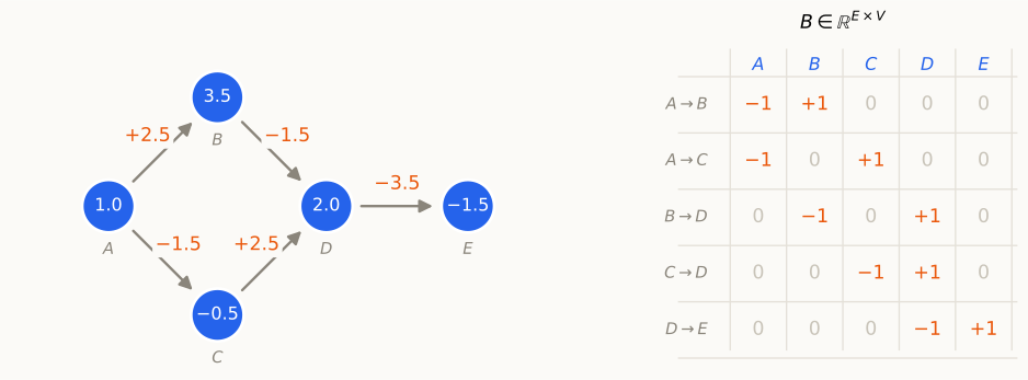
Blue = \(f\) at each vertex; orange = \((\nabla f)(e) = f(j)-f(i)\) on each oriented edge. Each row of \(B\) is \(-1\) at the tail, \(+1\) at the head: \((Bf)_e = (\nabla f)(e)\).

The flow \(\nabla f \in \mathbb{R}^E\) can be thought of as a vector field, i.e., a member of the tangent bundle, where \((\nabla f)_e\) represents the directional derivative of the function \(f\) along edge \(e\).

Divergence \(= -\nabla^*\), and the measure matters

In continuous space (e.g., on a smooth compact manifold \(M\) with no boundary), the adjoint of the gradient with respect to the standard \(L^2\) inner product is the negative divergence: \[ \int_M f\,(-\operatorname{div} X) \, dV = \int_M \langle \nabla f, X\rangle \, dV \]

To make this work on graphs, we need to define appropriate inner products on both the space of functions on vertices and the space of flows on edges.

	manifold	graph
on vector fields	metric \(g\)	edge weights: \(\langle X,Y\rangle_w = \sum_e w_e X_eY_e\)
on functions	volume \(dV\)	vertex measure \(m\): \(\langle f,g\rangle_m = \sum_i m_if_ig_i\)

Define \(\nabla^*_m\) by \(\langle\nabla f, X\rangle_w = \langle f,\nabla_m^*X\rangle_m\). Expanding, for coordinate \(i\):

\[ (\nabla_m^* X)_i = \frac{1}{m_i}\Big(\sum_{e \text{ into } i} w_eX_e - \sum_{e \text{ out of } i} w_eX_e\Big) =: -(\operatorname{div}_m X)_i . \]

Divergence = net weighted outflow per unit vertex mass.

Example: the divergence of \(\nabla f\)

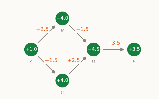
Green = \(\operatorname{div}(\nabla f)_i\) (counting measure, \(m\equiv1\), unweighted): outflow minus inflow at \(i\). E.g. at \(D\): \((-3.5) - \big((-1.5)+(2.5)\big) = -4.5\).

Like in continuous space, \(-\nabla^*\) measures the net outflow of a vector field per unit volume (or vertex mass, in the graph case).

Same graph and same flow X = grad f as two slides ago (orange edge labels unchanged). Now sum signed flow at each vertex: div(X)_i = sum of X_e over edges leaving i, minus sum of X_e over edges entering i. Check: the five div values sum to 0 (telescoping — every edge contributes +X_e to one endpoint and -X_e to the other). Also: div(grad f) = -Lf here, matching div = -nabla^* and L = nabla^* nabla for the counting measure, previewed on the next slide.

Both Laplacians are \(-\operatorname{div}\nabla\)

Proposition. \(\displaystyle(\nabla_m^*\nabla f)_i = \frac1{m_i}\sum_{j\sim i}w_{ij}(f_i - f_j)\). Hence

• \(m \equiv \mathbf 1\) (counting measure): \(\;\nabla^*\nabla = B^\top WB = D - A = L\), the combinatorial Laplacian;
• \(m = d\) (degree measure): \(\;\nabla_d^*\nabla = D^{-1}L = L_{rw}\), the random-walk Laplacian.

• Self-adjoint and PSD in \(L^2(m)\) for every \(m\) — nothing to check.
• The normalized Laplacian \(\mathcal L = D^{-1/2}LD^{-1/2}\) is \(L_{rw}\) moved to the unweighted space by the isometry \(f\mapsto D^{1/2}f\).

Lecture 1: “a change of which inner product, not a repair of a broken operator.” Now with a reason: the vertex measure is the volume form.

Proof: each edge between i and a neighbor j contributes w_ij (f_i - f_j) regardless of orientation (two cases: e into i or out of i).

Green’s identity and the Dirichlet form

By construction (“integration by parts”):

\[ \langle f,\nabla_m^*\nabla g\rangle_m = \langle\nabla f,\nabla g\rangle_w = \sum_{\{i,j\}\in E} w_{ij}\,(f_i - f_j)(g_i - g_j) \]

\[ \longleftrightarrow\qquad \int f\,(-\Delta g) = \int\langle\nabla f,\nabla g\rangle . \]

• No boundary term: graph Laplacians have Neumann boundary conditions built in.

With \(m = \mathbf 1\) (counting measure), we get the energy: \[\langle f,\nabla_m^*\nabla f\rangle_m = \langle\nabla f,\nabla f\rangle_w = \sum w_{ij}(f_i-f_j)^2 \leftrightarrow \int|\nabla f|^2\]

With \(m = \pi\), \(\pi_i = d_i/\mathrm{vol}(V)\), the normalized degree distribution, we get the Dirichlet form:

\[ \mathcal E(f,g) := \langle f, L_{rw}g\rangle_\pi = \frac{1}{\mathrm{vol}(V)}\sum_{\{i,j\}\in E} w_{ij}(f_i-f_j)(g_i-g_j). \]

Dictionary

Riemannian manifold \((M,g)\)	weighted graph \(G = (V,E,w)\)
metric \(g\) (conductivity)	edge weights \(w\)
volume measure \(dV\)	vertex measure \(m\) (counting, or degree)
\(\operatorname{div} = -\nabla^*\)	\(\operatorname{div}_m = -\nabla_m^*\)
\(\Delta = -\operatorname{div}\nabla \succeq 0\)	\(L\) (\(m=\mathbf 1\)), \(\;L_{rw}\) (\(m = d\))
\(\int_M|\nabla f|^2\,dV\)	\(\sum_{ij}w_{ij}(f_i-f_j)^2\)
Neumann boundary conditions	automatic
weighted manifold \((M,g,e^{-U}dV)\): \(\;\Delta_U = -e^{U}\operatorname{div}(e^{-U}\nabla\,\cdot)\)	\(L_{rw}\), self-adjoint in \(L^2(\pi)\)
Poincaré: \(\operatorname{Var}(f)\le C\int|\nabla f|^2\)	\(\operatorname{Var}_\pi(f)\le\lambda^{-1}\mathcal E(f,f)\) (soon)

For later:Weighted-manifold row: \(\Delta_U\) is (minus) the generator of Langevin diffusion with stationary density \(\propto e^{-U}\). \(L_{rw}\) is its discrete twin, with \(\pi\propto d\) playing \(e^{-U}\).

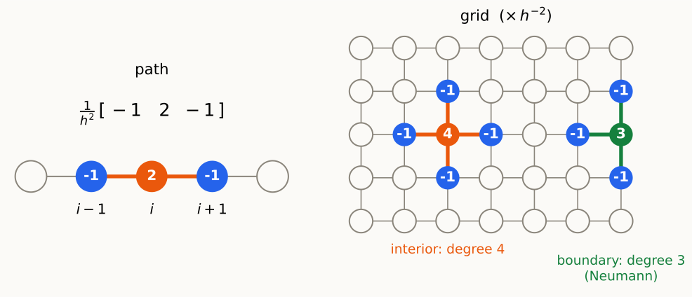
Sanity check: finite differences

• Path, weights \(h^{-2}\): \(\;(Lf)_i = h^{-2}(2f_i - f_{i-1} - f_{i+1})\to -f''\) — the 3-point stencil.
• Grid, weights \(h^{-2}\): \(\;(Lf)_{i,j} = h^{-2}(4f_{i,j} - f_{i\pm1,j} - f_{i,j\pm1})\to-\Delta f\) — the 5-point stencil.

Interior grid vertex: degree 4, so L is exactly the 5-point stencil for −Δ. Boundary vertex (green): degree 3; L drops the missing term, equivalent to a ghost value equal to the vertex’s own value, i.e. zero normal derivative (Neumann). Dirichlet would keep the diagonal at 4/h² and lose 1 from the kernel. The cycle’s spectrum (sampled Fourier modes) is computed in Lecture 3, §4.

Recap: properties of the Laplacian

Both \(L\) and \(L_{rw}\) — any \(\nabla_m^*\nabla\) — share three structural facts, for free:

1. Self-adjoint in \(L^2(m)\), for every \(m\): \(L = \nabla_m^*\nabla\) has the form \(A^*A\).

2. Positive semi-definite. \(\langle f,Lf\rangle_m = \langle\nabla f,\nabla f\rangle_w = \sum_{ij}w_{ij}(f_i-f_j)^2\ge0\).

3. Spectrum is bounded. \(G\) connected \(\Rightarrow\) \(0=\lambda_1<\lambda_2\le\cdots\le\lambda_n\), with \(\ker L = \operatorname{span}(\mathbf 1)\) (\(\lambda_1\) simple). Upper end: \(\lambda_n(L)\le 2d_{\max}\) (Gershgorin); for \(L_{rw}\) and \(\mathcal L\) (\(m=d\)), which are similar to each other: \(\lambda_n\le 2\).

Self-adjoint + PSD + bounded spectrum \(\Rightarrow\) an orthonormal eigenbasis and a well-behaved heat kernel \(H_t = e^{-tL_{rw}}\) — exactly what the rest of this lecture, and the next, leans on.

(1)-(2) are immediate from the A*A form shown on the “Both Laplacians” slide — nothing new to check for any m or any edge weights. (3): kernel = constants because G is connected (gradient slide, §1). Gershgorin for the upper bound: row i of L has diagonal d_i and off-diagonal entries summing to d_i in absolute value, so every eigenvalue lies in some disc [0, 2d_i], hence lambda_n <= 2 d_max. For L_rw = D^{-1}L (similar to the symmetric L = D^{-1/2} L D^{-1/2}), the same argument with row sums of L_rw equal to 1 gives lambda_n <= 2 directly — this is the bound quoted later (spectral decomposition slide, §2). This slide is pure bookkeeping — the content is all already on screen earlier, just gathered in one place before we start using it.

§2 · The random walk and measure/function duality

The random walk transition matrix

At each step, the random walk picks a neighbor with probability proportional to the edge weight. The probability transition matrix is: \[P = D^{-1}A, \quad P_{ij} = \Pr[X_{t+1}=j\mid X_t = i] = w_{ij}/d_i.\]

Stationary distribution is \(\pi_i = d_i/\mathrm{vol}(V)\): \[\pi^\top P = \pi^\top D^{-1}A = \frac{1}{\mathrm{vol}(V)}\mathbf 1^\top A = \frac{1}{\mathrm{vol}(V)}\mathbf 1^\top D = \pi^\top.\]

One matrix, two actions

Measures (row vectors)

\[\mu^\top\ \mapsto\ \mu^\top P\]

law of \(X_1\) when \(X_0\sim\mu\)

Functions (column vectors)

\[(Pf)(i) = \mathbb E[f(X_1)\mid X_0 = i]\]

local averaging

Canoical pairing \(\langle\mu,f\rangle = \mu^\top f = \mathbb E_\mu f\):

\[ \langle\mu^\top P, f\rangle = \mu^\top Pf = \langle\mu, Pf\rangle . \]

Evolve the distribution forward and observe, or evolve the observable and average against the start. Same number.

Continuous time: heat kernel

Jump at the rings of a rate-1 Poisson clock:

\[ H_t = \sum_{k\ge0}e^{-t}\frac{t^k}{k!}P^k = e^{-t(I-P)} = e^{-tL_{rw}},\qquad (H_tf)(i) = \mathbb E_i f(X_t). \]

• Backward (functions): \(\partial_tf_t = -L_{rw}f_t\) — Lecture 1’s heat equation.
• Forward (measures): \(\mu_t^\top = \mu_0^\top H_t\), \(\;\partial_t\mu_t^\top = -\mu_t^\top L_{rw}\) — master / Fokker–Planck.

Semigroups and generators

We will see that the heat kernel is the special case of a semigroup:

Definition (Semigroup): A family of operators \(\{H_t\}_{t\ge0}\) is a semigroup if:

• \(H_0 = I\), and
• \(H_{s+t} = H_s H_t\) for all \(s,t\ge0\).

Generator (Markov convention): The generator \(\mathcal{A}\) describes the infinitesimal evolution of the semigroup:

\[\mathcal A = \frac{d}{dt}H_t\big|_{t=0} = P - I = -L_{rw}\]

Sign: we keep the positive operator L_rw ⪰ 0 to match Δ = −div∇ ⪰ 0 from Lecture 1; Markov literature calls A = −L_rw the generator. Semigroup properties used later: H_0 = I, H_{s+t} = H_s H_t, H_t 1 = 1, positivity. Everything below uses only these + self-adjointness, which is why it transfers to diffusions.

Advantages of Continuous Time

• Can differentiate by time: \(\partial_t H_t = -L_{rw} H_t\).
• Avoids the bipartite problem: eigenvalues of \(H_t\) are in \((0,1]\) rather than \(P\) having \(-1\).

Cycle (\(n\) even), grid, binary tree: all bipartite \(\Rightarrow\) \(P\) has eigenvalue \(-1\).

The discrete walk from a vertex never converges — it alternates sides.

This problem can alternatively be fixed by making the walk lazy:

\[P_{\rm lazy} = \tfrac12(I + P) = I - \tfrac12L_{rw}\],

This has eigenvalues \(1 - \tfrac{\lambda_k}{2}\in[0,1]\).

We work in continuous time; discrete-time statements follow with \(e^{-\lambda}\to 1-\lambda/2\).

Stationarity and detailed balance

Question: What does self-adjointness in \(L^2(\pi)\) imply for the behavior of the random walk?

Detailed balance:

\[ \pi_iP_{ij} = \frac{w_{ij}}{\mathrm{vol}(V)} = \pi_jP_{ji}\qquad\Longleftrightarrow\qquad\Pi P = P^\top\Pi,\quad\Pi = \operatorname{diag}(\pi). \]

\(\Longleftrightarrow\) \(P\), \(L_{rw}\), \(H_t\) are self-adjoint in \(L^2(\pi)\):

\[ \langle f, Pg\rangle_\pi = f^\top\Pi Pg = f^\top P^\top\Pi g = \langle Pf, g\rangle_\pi . \]

Same fact as \(\nabla_\pi^*\nabla = \mathrm{vol}(V)\,L_{rw}\), now seen probabilistically.

Densities are functions

Write \(\mu = \Pi h\), i.e. \(h = d\mu/d\pi\), \(\;h_i = \mu_i/\pi_i\).

Proposition. If \(\mu_t^\top = \mu_0^\top H_t\) then \(h_t = H_t^*h_0\), with \(H_t^* = \Pi^{-1}H_t^\top\Pi\) the adjoint in \(L^2(\pi)\). For reversible walks \(H_t^* = H_t\): \[h_t = H_th_0 .\] Densities obey the same heat equation as observables.

Proof. \(h_t = \Pi^{-1}H_t^\top\Pi h_0\), and \(\langle f,\Pi^{-1}H_t^\top\Pi g\rangle_\pi = f^\top H_t^\top\Pi g = \langle H_tf,g\rangle_\pi\). Detailed balance: \(\Pi H_t = H_t^\top\Pi\). \(\square\)

• \(\mu\mapsto\mu/\pi\) is an isometry from \((\mathbb R^V,\langle\cdot,\cdot\rangle_{1/\pi})\) (measures) to \(L^2(\pi)\) (functions): the Riesz map.
• Non-reversible chains: \(h_t\) evolves by the time-reversed semigroup. We’ll meet this again with general Markov semigroups.

Demo: measures vs densities — split and aggregate

open in new tab ↗

One loop: vertex mass –D⁻¹–> value on each edge-end –send–> far end –A–> vertex mass. Measures and densities are the same loop cut at different places. Measures (start at red vertex mass): split (D⁻¹), send, aggregate (A): μᵀ ↦ μᵀD⁻¹A = μᵀP. Mass is conserved. Densities (start at blue value, x = D⁻¹μ = h/vol): send copies, aggregate (A), average (D⁻¹): x ↦ D⁻¹Ax = Px. Constants are preserved. Point out: in density mode the red intermediate Ax_t is exactly μ_{t+1}; the invariant μ_t = D x_t holds at every step. Run it: μ_t → π ∝ degree (uneven red bars), x_t → constant 1/vol (flat blue bars). This makes the previous two slides concrete: π is the fixed point of the measure loop, and densities evolve by the same P as functions (they converge to constants). Graph and starting values are from the old SGT figure (degrees 1,3,2,2; vol = 8). It has a triangle, so the discrete walk is aperiodic and converges.

Spectral decomposition and the Poincaré inequality

\(L_{rw}\) self-adjoint in \(L^2(\pi)\) \(\Rightarrow\) orthonormal eigenbasis \(\varphi_1 = \mathbf 1,\varphi_2,\dots,\varphi_n\), \(\;0=\lambda_1<\lambda_2\le\dots\le\lambda_n\le2\):

\[ H_tf = \sum_ke^{-\lambda_kt}\langle f,\varphi_k\rangle_\pi\varphi_k,\qquad \mathcal E(f,f) = \sum_k\lambda_k\langle f,\varphi_k\rangle_\pi^2, \]

\[ \operatorname{Var}_\pi(f) = \sum_{k\ge2}\langle f,\varphi_k\rangle_\pi^2 . \]

Spectral gap \(\lambda := \lambda_2(L_{rw})\). Courant–Fischer:

\[ \lambda = \min_{f\ \text{non-const}}\frac{\mathcal E(f,f)}{\operatorname{Var}_\pi(f)} \quad\Longleftrightarrow\quad \boxed{\ \lambda\operatorname{Var}_\pi(f)\le\mathcal E(f,f)\ } \]

Poincaré inequality: “small gradient \(\Rightarrow\) nearly constant.” Relaxation time \(t_{\rm rel} := 1/\lambda\).

The variance is an energy too. \(\operatorname{Var}_\pi(f) = \sum_{a<b}\pi_a\pi_b(f_a-f_b)^2 = \frac{1}{\mathrm{vol}(V)}\sum_{a<b}\frac{d_ad_b}{\mathrm{vol}(V)}(f_a-f_b)^2 = \mathcal E_{K_G}(f,f)\), the energy of the complete graph \(K_G\) with weights \(w'_{ab} = d_ad_b/\mathrm{vol}(V)\), which has the same degrees as \(G\) (counting self-loops). So Poincaré is a comparison of two graphs: \(\lambda\,L_{K_G}\preceq L_G\).

Degrees of K_G: Σ_b d_a d_b / vol = d_a (the b = a term is a self-loop, invisible to the energy). K_G has the same stationary distribution π, and its walk is P’ = 1π^T: it jumps straight to stationarity in one step. So λ measures how well G approximates the “ideal mixer” with the same degrees. This K_G is the graph from the old SGT notes (“why Laplacians?”).

Takeaways

• \(L\), \(L_{rw}\): the same \(-\operatorname{div}\nabla\) with different volume measures. Self-adjointness and PSD are automatic.
• The walk \(P = D^{-1}A\) acts on measures (row vectors, \(\mu^\top P\)) and on functions (column vectors, \(Pf\)); continuous time gives the heat kernel \(H_t = e^{-tL_{rw}}\) with generator \(-L_{rw}\).
• Detailed balance \(\Leftrightarrow\) \(L_{rw}\) self-adjoint in \(L^2(\pi)\) \(\Rightarrow\) densities \(h = \mu/\pi\) evolve like functions: \(h_t = H_th_0\).
• Spectral gap \(\lambda = \lambda_2(L_{rw})\) = best Poincaré constant, \(\lambda\operatorname{Var}_\pi(f)\le\mathcal E(f,f)\).
• Next: measuring convergence to \(\pi\), and what the gap says about mixing times.

Appendix: definitions for the board

Operators and the walk

Graph. \(G = (V,E,w)\) undirected, connected; \(d_i = \sum_jw_{ij}\); \(\mathrm{vol}(S) = \sum_{i\in S}d_i\); \(\pi_i = d_i/\mathrm{vol}(V)\), \(\Pi = \operatorname{diag}(\pi)\).

Gradient / divergence. \((\nabla f)(i\to j) = f_j - f_i\); \(\operatorname{div}_m = -\nabla_m^*\) w.r.t. \(\langle\cdot,\cdot\rangle_w\) on edges and \(\langle\cdot,\cdot\rangle_m\) on vertices. \(\nabla^*\nabla = L = D-A\); \(\nabla_d^*\nabla = L_{rw} = D^{-1}L = I-P\); \(\mathcal L = D^{-1/2}LD^{-1/2}\).

Dirichlet form. \(\mathcal E(f,g) = \langle f,L_{rw}g\rangle_\pi = \frac1{\mathrm{vol}(V)}\sum_{\{i,j\}\in E}w_{ij}(f_i-f_j)(g_i-g_j)\).

Walk. \(P = D^{-1}A\); measures \(\mu^\top P\), functions \(Pf\). Random-walk Laplacian \(L_{rw} = I - P\). Continuous time \(H_t = e^{-tL_{rw}}\), generator \(\mathcal A = P - I = -L_{rw}\). Lazy: \(P_{\rm lazy} = \frac12(I+P)\).

Reversibility. \(\Pi P = P^\top\Pi\); densities \(h = \mu/\pi\) evolve as \(h_t = H_th_0\).

Gap / Poincaré. \(\lambda = \lambda_2(L_{rw}) = \min_f\mathcal E(f,f)/\operatorname{Var}_\pi(f)\); \(t_{\rm rel} = 1/\lambda\).