Why Eigenvectors?

A tour of spectral methods

CMSC 35410 · Lecture 1

§0 Course overview

Motivation

Spectral methods are a powerful tool for understanding complex systems by studying the eigenvalues and eigenvectors of associated linear operators. Because their theory generalizes from finite-dimensional linear algebra to infinite-dimensional settings, they provide a unifying framework for the analysis and computation of a wide range of problems.

Tentative Topic List: Spectral methods in finite dimensions

• Spectral Graph Theory
• Random Walks Over Graphs and Their Convergence
• Spectral Clustering
• Cheeger’s Inequality
• Modern Spectral Algorithms via Semidefinite Programming
• Spectral Sparsification
• Expander Graphs and Their Significance
• Markov Chains Mixing Times and Log-Sobolev Inequalities
• Method of Moments for Latent-Variable Models

Tentative Topic List: Spectral methods in infinite dimensions

• Sturm-Liouville Theory and Spectral Decomposition
• Markov Processes in Continuous Space and Their Generators
• Brownian Motion and the Laplacian
• Langevin Dynamics and the Fokker-Planck Equation
• Bakry-Emery Theory
• Manifold Learning and Diffusion Maps
• Spectral Collocation Methods

Eigenvectors, Eigenvalues and Diagonalization

Definition: An eigenvector of a matrix \(A\) is a nonzero vector \(\mathbf{v}\) such that

\[ A \mathbf{v} = \lambda \mathbf{v} \] for some scalar \(\lambda\), called the eigenvalue corresponding to \(\mathbf{v}\).

Spectral Decomposition: A matrix \(A\) is diagonalizable if it can be written as

\[ A = V \Lambda V^{-1}, \] where the columns of \(V\) are the eigenvectors of \(A\) and \(\Lambda\) is a diagonal matrix containing the corresponding eigenvalues.

NB1: Not all matrices are diagonalizable. In such cases, we may need to consider generalized eigenvectors and the Jordan canonical form.

NB2: When \(A\) is symmetric, it is always diagonalizable with an orthonormal set of eigenvectors.

Why Eigenvectors and Eigenvalues Matter

Variational Interpretation:Eigenvectors and eigenvalues are solutions of optimization problems:

\[ \lambda_{\max}(A) = \max_{\mathbf{v} \neq 0} \frac{\mathbf{v}^\top A \mathbf{v}}{\mathbf{v}^\top \mathbf{v}} \]

This can be generalized to other eigenvalues and their corresponding eigenvectors (see the Courant-Fischer min-max theorem in review notes).

Geometric Interpretation: Eigenvectors indicate directions in which the linear transformation associated with the matrix acts by simply scaling, and the corresponding eigenvalues indicate the scaling factor.

For a symmetric matrix \(A\): \[ A = Q \Lambda Q^\top = \sum_{i=1}^n \lambda_i \mathbf{q}_i \mathbf{q}_i^\top, \] a weighted sum of projections onto the eigenvectors.

Why Eigenvectors and Eigenvalues Matter 2

Variational Interpretation:Eigenvectors and eigenvalues are solutions of optimization problems.

Geometric Interpretation: Eigenvectors indicate directions in which the linear transformation associated with the matrix acts by simply scaling, and the corresponding eigenvalues indicate the scaling factor.

Algebraic Interpretation: Eigenvectors and eigenvalues provide a way to understand the structure of a matrix through its diagonalization, revealing invariant subspaces and simplifying matrix computations.

\[ A^t \mathbf{u} = Q \lambda^t Q^{-1} \mathbf{u} \] This is super-useful for solving linear ODEs: \[ \mathbf{\dot{x}}(t) = A \mathbf{x}(t) \to \mathbf{x}(t) = e^{At} \mathbf{x}(0) = Q e^{\Lambda t} Q^{-1} \mathbf{x}(0). \]

Show of hands

• Who has used PCA?
• Who has run a clustering algorithm?
• Who has, today, typed something into a search engine?

Everyone here has already used a spectral method today, probably without the label.

~2 min. The pitch for the whole course: this is a move you already rely on.

The strategy this course is about

Take something that looks intractable (combinatorial, continuous, noisy) and turn it into “compute the eigenvalues / eigenvectors of some linear operator.”

Today’s tour visits communities that rarely read each other’s papers:

	Community	Operator
§1	Web search	Google matrix \(M\) (not symmetric)
§2–3	Graph partitioning	Graph Laplacian \(L\), \(\mathcal L\)
§4	Statistics / ML	Covariance matrix, SVD
§5	Geometry / physics	Heat semigroup \(e^{-tL}\), Laplace–Beltrami \(\Delta\)
§6–7	Numerical analysis	Differential operators, Chebyshev / Fourier bases

§1 · The hook: PageRank

A random surfer

Web = directed graph \(G=(V,E)\). The surfer follows a random out-link, but with probability \(1-\alpha\) teleports to a uniformly random page:

\[ M \;=\; \alpha P + (1-\alpha)\,\tfrac1n \mathbf 1\mathbf 1^\top . \]

The PageRank vector is a left eigenvector with eigenvalue 1:

\[ \pi^\top M = \pi^\top . \]

Perron–Frobenius: \(M\) is strictly positive and stochastic, so \(\pi\) exists, is unique, and is entrywise positive.

§1 total ~12 min. Perron–Frobenius (informal): strictly positive irreducible matrix ⇒ real, simple, largest-modulus eigenvalue with positive eigenvector.

The algorithm is the eigenvector computation

Power iteration: \(\;\pi_{k+1}^\top = \pi_k^\top M\).

Why it converges: teleportation is a contraction in \(\ell_1\). A difference of probability vectors sums to \(0\), so the teleport term drops out:

\[ \|\pi_{k+1} - \pi\|_1 = \alpha\,\big\|(\pi_k - \pi)^\top P\big\|_1 \;\le\; \alpha\,\|\pi_k - \pi\|_1,\\ \qquad\text{so}\qquad \|\pi_k - \pi\|_1 \le 2\,\alpha^k . \]

Spectrally: \[\;\operatorname{spec}(M) = \{1\} \cup \alpha\cdot\{\lambda_2(P),\dots,\lambda_n(P)\},\] so the spectral gap is \(1 - |\lambda_2(M)| \ge 1 - \alpha\).

Discussion: what does a small spectral gap mean physically for the surfer?

Answer: slow mixing — the surfer’s distribution takes a long time to forget where it started. Same phenomenon as Markov chain mixing time; formalized with graph spectral gaps in a few weeks.

Contraction proof: for probability vectors \(x,y\), \(z = x-y\) has \(z^\top\mathbf 1 = 0\), so \(z^\top M = \alpha z^\top P + \tfrac{1-\alpha}{n}(z^\top\mathbf 1)\mathbf 1^\top = \alpha z^\top P\); \(P\) row-stochastic gives \(\|z^\top P\|_1 \le \|z\|_1\). Apply with \(x = \pi_k\), \(y = \pi\).

Eigenvalue proof (Haveliwala–Kamvar 2003): if \(x^\top M = \lambda x^\top\) with \(\lambda \ne 1\), then \(M\mathbf 1 = \mathbf 1\) forces \(x^\top\mathbf 1 = 0\), hence \(x^\top P = (\lambda/\alpha)x^\top\), so \(|\lambda| \le \alpha\). Equality iff \(P\) has a second unimodular eigenvalue (e.g. two closed components). Assumes dangling pages are patched so \(P\) is row-stochastic.

Why prefer the contraction: \(M\) is non-normal, so the eigenvalue bound only gives \(C|\lambda_2(M)|^k\) with \(C\) depending on eigenvector conditioning; the \(\ell_1\) argument has constant 1 and holds for every \(k\). That is the dashed \(\alpha^k\) line in the demo. Well-mixed graph: \(|\lambda_2(P)|\) small, so the error beats \(\alpha^k\) by a lot; two communities: \(\lambda_2(P) \approx 1\), error tracks \(\alpha^k\).

Demo: power iteration

open in new tab ↗

Run on the well-mixed web first (α = 0.85), then switch to “Two communities” and push α toward 0.97. The orange faint curve is the other graph at the same α. Point out: the αᵏ line is only an upper bound — the well-mixed graph beats it by a lot, the two-community graph barely does.

A remark to flag now, pay off later

\(M\) comes from a directed graph, so it is generally

• not symmetric,
• not even normal (\(MM^* \neq M^*M\)),
• with left and right eigenvectors that differ.

No inner product makes it self-adjoint: no diagonal reweighting enforces detailed balance on a generic directed graph.

Perron–Frobenius still gives a real, positive dominant eigenvalue — but the clean orthogonal-eigenbasis picture of the spectral theorem is not operating here.

Hold that thought — it resurfaces in §2, in reverse.

§2 · From graphs to eigenvectors: spectral clustering

Partitioning a graph

Weighted undirected graph, adjacency \(A\), degrees \(D\), Laplacian

\[ L = D - A, \qquad x^\top L x = \sum_{(i,j)\in E} w_{ij}(x_i - x_j)^2 \;\ge 0, \qquad L\mathbf 1 = 0 . \]

Goal: clusters with few crossing edges (Conductance/Normalized Cut Objective). NP-hard as stated.

Relax the \(\pm1\) indicator to any real vector:

\[ \min_{\mathbf{x}^\top D\mathbf 1 = 0}\; \frac{\mathbf{x}^\top L \mathbf{x}}{\mathbf{x}^\top D \mathbf{x}} \;=\; \lambda_2(L), \]

attained exactly by the Fiedler vector \(v_2\).

§2 total ~15 min. The Rayleigh quotient on the board: extrema over the unit sphere are the extreme eigenvalues; Courant–Fischer gives the rest.

Demo: thresholding the Fiedler vector

open in new tab ↗

Start in “True layout”. Then “Scrambled” — the algorithm never saw the geometry, only the edges; colors still separate the blobs. Then “Ordered by Fiedler”. Increase bridge weight / count: λ₂ grows, the gap to λ₃ closes, clustering gets worse. The Cheeger readout at the bottom previews §3.

Self-adjointness, precisely

For any undirected weighted graph (no regularity needed):

• \(L_{rw} = D^{-1}L\) and \(P = D^{-1}A\) are self-adjoint w.r.t. \(\langle x,y\rangle_D = x^\top D y\) — this is exactly detailed balance for \(\pi \propto \deg\);
• \(\mathcal L = D^{1/2} L_{rw} D^{-1/2}\) is the same operator, self-adjoint w.r.t. the standard inner product.

A change of which inner product you measure against — not a repair of a broken operator. Undirected graphs get this for free; directed graphs (§1) generally do not.

This is Exercise 4 in the Linear Algebra Review note — assign before or after this lecture.

§3 · A real theorem: Cheeger’s inequality

An eigenvalue certifies a bottleneck

Conductance of \(G\): \[ h(G) = \min_{S}\; \frac{|\partial S|}{\min\big(\mathrm{vol}(S),\, \mathrm{vol}(V\setminus S)\big)} . \]

Cheeger’s inequality. With \(\lambda_2\) the second-smallest eigenvalue of \(\mathcal L\),

\[ \frac{\lambda_2}{2} \;\le\; h(G) \;\le\; \sqrt{2\lambda_2} . \]

• Not a heuristic: a two-sided, provable certificate.
• The upper bound is constructive: a sweep cut of \(D^{-1/2}v_2\) achieves it (the dashed line in the demo).
• Proof later in the term; then SDP relaxations (ARV) and sparsification (Spielman–Teng).

~10 min. Goal today is the shape of the result, not the proof. Fill in the week number for the proof.

§4 · The bridge everyone already knows: PCA / SVD

The spectral theorem

PCA computes eigenvectors of the (symmetric, PSD) covariance matrix. Time to state what §2–3 were quietly leaning on:

Spectral theorem. If \(A = A^*\) on an \(n\)-dimensional inner product space, there is an orthonormal basis \(v_1,\dots,v_n\) of eigenvectors with real eigenvalues: \[A = Q\Lambda Q^*, \qquad Q \text{ unitary}.\]

SVD is the rectangular generalization: \(A = U\Sigma V^*\).

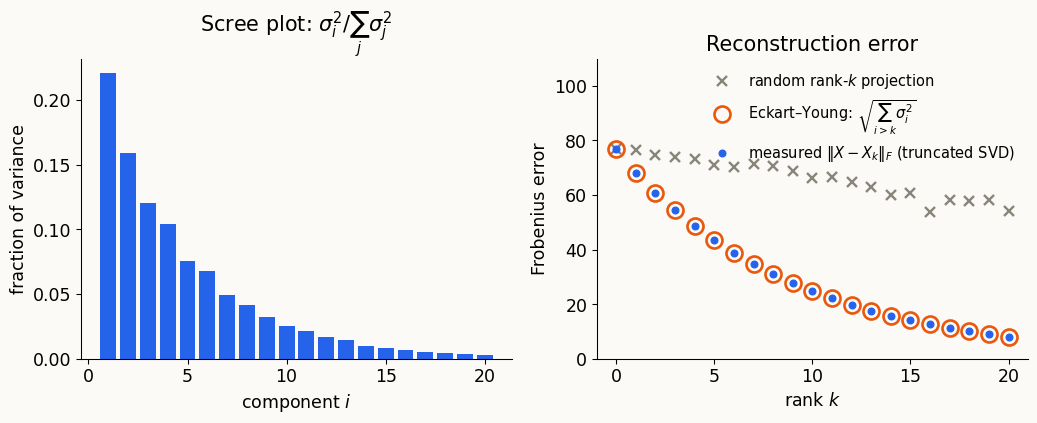
Eckart–Young. \(A_k = \sum_{i\le k} \sigma_i u_i v_i^*\) is the best rank-\(k\) approximation in Frobenius and operator norm: \(\;\|A - A_k\|_F^2 = \sum_{i>k}\sigma_i^2 .\)

§4 total ~12 min. This is the result every student has used via sklearn without knowing it’s a spectral-theorem statement dressed up.

Demo: PCA on synthetic data

Blue dots sit exactly on the orange line: the reconstruction error is predicted by the discarded singular values, and nothing of rank k does better (grey = random subspace).

The framing line

“Every example so far that behaved nicely — orthogonal eigenvectors, real eigenvalues, stable numerics — was secretly symmetric, or could be made symmetric. PageRank’s matrix was not, and we saw the clean picture partially break. Much of this course is about knowing which case you’re in before you start computing.”

§5 · Diffusion and the shape of things

Heat on a graph

\[ \frac{du}{dt} = -Lu,\quad u(0)=u_0 \qquad\Longrightarrow\qquad u(t) = \sum_k e^{-\lambda_k t}\,\langle u_0, v_k\rangle\, v_k . \]

• \(\lambda_1 = 0\): the constant mode survives forever (equilibrium).
• Every other mode decays at its own rate \(e^{-\lambda_k t}\).
• The slowest non-constant mode is \(v_2\) — the Fiedler vector again.

Same eigenvector, two jobs: “the best 2-way cut” and “the last non-uniform heat left before equilibrium.”

§5 total ~12–15 min. Loosely follows the opening of Rosenberg, The Laplacian on a Riemannian Manifold. Qualitative today.

Demo: watching heat diffuse

open in new tab ↗

Cycle first: press Play; the blue curve is the continuous heat kernel on a circle of the same length (Fourier eigenbasis) — discrete and continuous agree once the high modes are gone. Then “Two clusters + bridge”: after the high modes die, what remains is exactly the orange Fiedler mode — one cluster warm, the other cool. Path: slowest of all (λ₂ ≈ π²/n²).

From graphs to manifolds

Replace the graph by a compact Riemannian manifold \((M,g)\) and \(L\) by the Laplace–Beltrami operator \(\Delta = -\operatorname{div}\operatorname{grad}\):

• self-adjoint, \(\Delta \succeq 0\), discrete spectrum \(0 = \lambda_1 < \lambda_2 \le \cdots \to \infty\);
• eigenfunctions \(\phi_k\) form an orthonormal basis of \(L^2(M)\).

Heat equation \(\partial_t u = -\Delta u\), solved by the heat kernel

\[ K(t,x,y) = \sum_k e^{-\lambda_k t}\,\phi_k(x)\,\phi_k(y). \]

The same equation as the graph case — a finite sum becomes a discrete-but-infinite one.

The eigenbasis comes from Theorem 7.1 in Linear Algebra Review, Part II (see its Section 8), applied to the compact self-adjoint resolvent (I+Δ)⁻¹.

Where the geometry hides

Heat trace, as \(t \to 0^+\) (Minakshisundaram–Pleijel):

\[ Z(t) = \sum_k e^{-\lambda_k t} \;\sim\; (4\pi t)^{-n/2}\Big(\mathrm{Vol}(M) + \tfrac{t}{6}\!\int_M \mathrm{Scal}\,dV + O(t^2)\Big). \]

From the list of eigenvalues alone you read off:

• the dimension \(n\) (rate of blow-up),
• the volume (leading coefficient),
• the total scalar curvature (next coefficient).

Weyl’s law, from the other end: \[N(\lambda) = \#\{k: \lambda_k \le \lambda\} \;\sim\; \frac{\omega_n \mathrm{Vol}(M)}{(2\pi)^n}\,\lambda^{n/2}.\]

Can one hear the shape of a drum?

Kac (1966): a drum’s shape determines its frequencies. Can you run that backward?

Gordon–Webb–Wolpert (1992): no. Two non-isometric planar drums with identical spectra.

The spectrum determines a great deal (dimension, volume, curvature, bottlenecks, …) — but not everything. Where exactly the line falls is a theme we return to.

Either way, actually computing with a continuous operator like \(\Delta\) is a real numerical problem. →

“Spectral” for eigenvalue problems comes from the analogy with spectral lines in physics.

§6 · Spectral methods for differential equations

Same word, different community

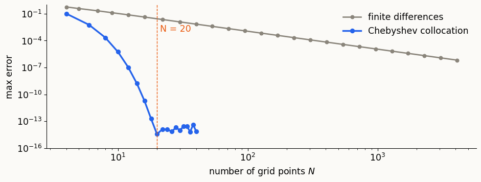
Solve \(\;u'' = e^{4x}\) on \([-1,1]\), \(\;u(\pm1)=0\).

• Finite differences: local stencils, error \(O(N^{-2})\).
• Chebyshev collocation: global polynomial basis, error \(O(\rho^{-N})\) for smooth \(u\) — “spectral” convergence.

§6 ~15 min. The intended “wow”: ~20 Chebyshev points reach machine precision; finite differences with thousands of points are still around 1e-6. Mention Orr–Sommerfeld (next slide) as a name-drop.

Planting a seed: non-normal operators

The Orr–Sommerfeld operator (hydrodynamic stability) is not self-adjoint.

• Eigenvalues alone can badly mislead about its behavior.
• Transient growth, sensitivity to perturbation → pseudospectra.

Same warning as PageRank, now for differential operators. We return to this once we have the machinery.

§7 · Payoff: spectral methods run the weather

Spherical harmonics and the global forecast

Operational global forecasting has long used the spectral transform method: expand fields in spherical harmonics (eigenfunctions of \(\Delta\) on \(S^2\)).

• Smooth global fields ⇒ exponential convergence (as in §6).
• A modest number of degrees of freedom buys enormous accuracy.

Not a classroom curiosity: part of why a global forecast is computationally tractable at all.

~5 min. Currency check before lecture: confirm current operational models’ numerics before citing specifics (e.g. ECMWF IFS), since this has been an active area of change.

Roadmap for the semester

• Spectral graph theory proper: expanders, mixing times, Cheeger’s inequality (proved).
• Spectral algorithms in ML: clustering, embeddings, low-rank models, diffusion maps.
• The recurring question underneath all of it:

What do we actually need — self-adjointness, normality, or just diagonalizability — and what breaks when we don’t have it?

PageRank and directed graphs were today’s first data point. More will come.

Appendix: definitions for the board

Operators and the spectral theorem

Inner product / adjoint. On \(\mathbb F^n\), \(\langle x,y\rangle = y^*x\). The adjoint satisfies \(\langle Ax,y\rangle = \langle x,A^*y\rangle\). \(A\) is self-adjoint if \(A=A^*\); normal if \(AA^* = A^*A\) (orthonormal eigenbasis, possibly complex eigenvalues).

Spectral theorem. \(A=A^*\) on an \(n\)-dim inner product space ⇒ orthonormal eigenbasis, real eigenvalues \(\lambda_1\ge\dots\ge\lambda_n\); \(A = Q\Lambda Q^*\).

Rayleigh quotient. \(R_A(x) = \langle Ax,x\rangle / \langle x,x\rangle\); extrema on the unit sphere are the extreme eigenvalues (Courant–Fischer gives the rest).

Perron–Frobenius (informal). Strictly positive irreducible matrix ⇒ real, simple, largest-in-modulus eigenvalue with a strictly positive eigenvector.

SVD / Eckart–Young. \(A = U\Sigma V^*\); \(A_k = \sum_{i\le k}\sigma_i u_i v_i^*\) is the best rank-\(k\) approximation in Frobenius and operator norm.

Graphs

For \(G=(V,E,w)\) undirected, symmetric adjacency \(A\), \(D = \mathrm{diag}(\deg)\):

• \(L = D - A\): symmetric, PSD, \(\mathbf 1\in\ker L\).
• \(L_{rw} = D^{-1}L\), \(\;P = D^{-1}A\).
• \(\mathcal L = D^{-1/2}LD^{-1/2} = I - D^{-1/2}AD^{-1/2}\).

Degree-weighted inner product \(\langle x,y\rangle_D = x^\top D y\): \(L_{rw}\) and \(P\) are self-adjoint w.r.t. it; \(\mathcal L = D^{1/2}L_{rw}D^{-1/2}\) is self-adjoint w.r.t. the standard one.

Conductance \(h(G) = \min_S |\partial S| / \min(\mathrm{vol}(S),\mathrm{vol}(V\setminus S))\). Cheeger: \(\lambda_2(\mathcal L)/2 \le h(G) \le \sqrt{2\lambda_2(\mathcal L)}\).

Heat semigroup. \(u(t) = e^{-tL}u_0 = \sum_k e^{-\lambda_k t}\langle u_0,v_k\rangle v_k\); kernel \(K_t = \sum_k e^{-\lambda_k t}v_kv_k^\top\).

Manifolds and numerics

Laplace–Beltrami. On compact \((M,g)\), \(\Delta = -\operatorname{div}\operatorname{grad}\) is self-adjoint, \(\Delta\succeq0\), spectrum \(0=\lambda_1<\lambda_2\le\cdots\to\infty\), eigenfunctions \(\phi_k\) an ONB of \(L^2(M)\). Heat kernel \(K(t,x,y) = \sum_k e^{-\lambda_k t}\phi_k(x)\phi_k(y)\).

Heat trace. \(Z(t) = \operatorname{Tr} e^{-t\Delta} \sim (4\pi t)^{-n/2}\big(\mathrm{Vol}(M) + \tfrac t6\int_M \mathrm{Scal}\,dV + O(t^2)\big)\).

Weyl’s law. \(N(\lambda) \sim \dfrac{\omega_n\mathrm{Vol}(M)}{(2\pi)^n}\lambda^{n/2}\).

Spectral convergence. For smooth data, global (Chebyshev/Fourier) bases converge faster than any power of \(1/N\); local finite-difference stencils converge at a fixed polynomial rate.